Spatial scaling - GRACE satellite data

The GRACE satellite data has been used for more than a decade to investigate the global-scale mass redistribution since April 2002. With the Follow-on mission which had recently (5/22/2018) been launched, the extended measurement is truly an important achievement in the field of Earth geodesy, hydrology, and cryosphere. To make use of this incredible dataset, there are three processing centers that offer all different kinds of GRACE solution. Each processing center generates the solution based on the range differences observed by the unique twin satellite setting. This also provides an opportunity for inter-comparison on the processing steps between solutions.

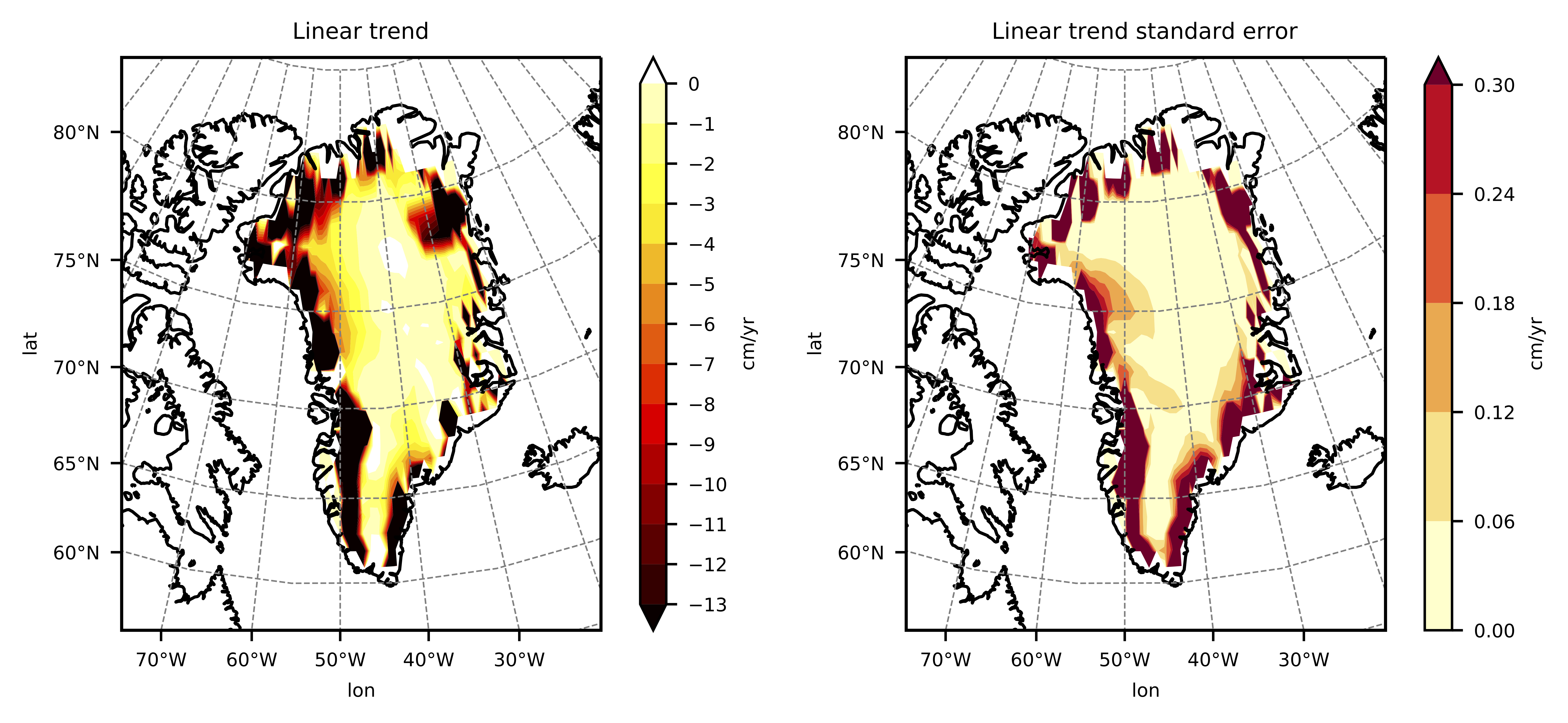
The signal in the GRACE satellite is usually smoothed out due to the various processing steps applied. This means that the signal would be distributed over a larger area despite the original signal is located over a much smaller area. To give you a sense of how a regular GRACE data is smoothed out, the following figure shows what we called the unscaled GRACE data over the Greenland region.

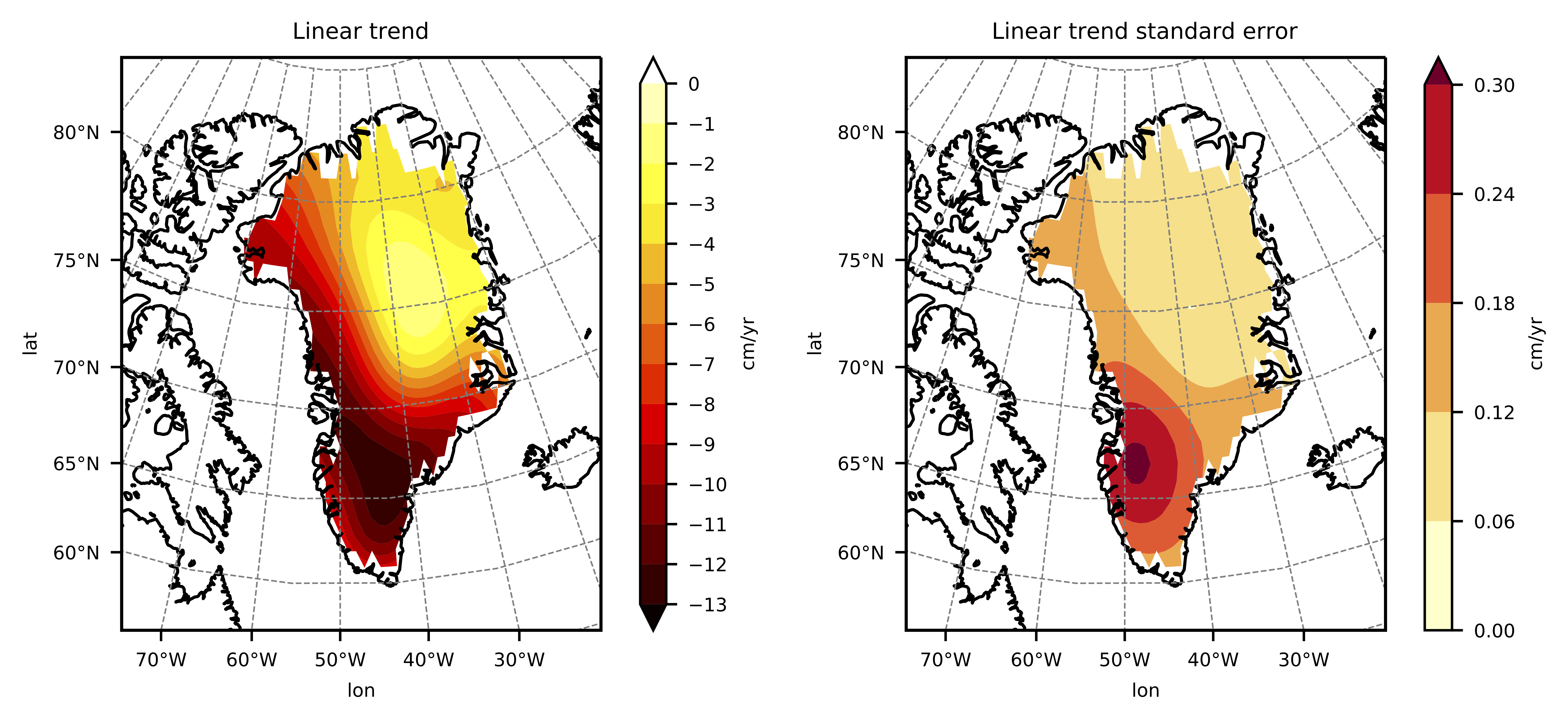
To overcome this smoothing problem in the GRACE data, I use the method described in my published paper [Hsu and Velicogna, 2017] to show how big the differences can be if one did not restore the signal properly. The following figure shows the scaled GRACE data over the same area.

Notice the large changes in maximum value which show in a saturated color. I intentionally make it saturate to keep the same colorbar scale so one can compare the two figures. You may also notice the shift of location of the maximum value. The maximum value is now located in the region which is much more reasonable than the unscaled (smoothed) GRACE data.

The concept of restoring the losing signal is to get the spatial information from a synthetic dataset. First, we applied the necessary processing steps on the synthetic dataset. Next, we calculate the univariate linear regression between the “processed synthetic data” and the “original synthetic data” to figure out the necessary scaling based on the regression coefficients [Landerer and Swenson, 2008]. This method generates a reasonable hydrological signal. However, the signal variation at different time scales can be dominated by separate physical processes. Single scaling provided by the previous study may only represent a single physical process that dominated the total signal. To improve the estimate in all timescale, we separated the signal to long-term variation and seasonal variation which we knew the dominated physical processes are different and perform multivariate linear regression. The multivariate linear regression provides us separate scaling factors for each timescale. By also separate the GRACE data to long-term variation and seasonal variation, we scale the GRACE signal at each time scale with its corresponding scaling factor.