Marine Heatwaves forecasting using NMME (North American Multi-Model Ensemble)

Predicting marine heatwaves

Using the NMME (North American Multi-Model Ensemble), Jacox et al., 2022 demonstrate the possibility of predicting the marine heatwaves under a monthly time scale with the lead time up to a year. The marine heatwaves portal forecast hosted at NOAA/PSL website is based on the calculation show in this notebook.

Goals in the notes

• Lazy loading the NMME model data from IRI/LDEO Climate Data Library

• Calculate the ensemble mean climatology for each model based on hindcast

• Calculate the SST anomaly in the forecast

• Calculate the threshold based on the SST anomaly

• Calculate the marine heatwave in the forecast

• Show result

Note

The following example is based on the paper Jacox et al., 2022.

Extract the data from the IRI/LDEO Climate Data Library OPeNDAP server

In this notebook, we demonstrate how to use the NMME model to generate the marine heatwaves prediction. The dataset is currently hosted on IRI/LDEO Climate Data Library.

Tip

The OPeNDAP server on the IRI/LDEO Climate Data Library also has a data extraction limit. For solving some of the limit issues, there are some great discussions on this GitHub issue. To summarize, user sometime will need to play a bit on the chunk size to find the optimal download scheme.

Import needed python package

import warnings
import cftime
import numpy as np
import xarray as xr
from dask.diagnostics import ProgressBar

warnings.simplefilter("ignore")

Tip

This line of code is not affecting the execution but just removing some warning outputs that might clutter your notebook. However, do pay attention to some of the warnings since they will indicate some deprecation of function and arg/kwarg in future software updates.

Lazy loading the NMME model data from IRI/LDEO Climate Data Library

Like in the previous notebook, we request the metadata from the OPeNDAP server to quickly check the data structure. Four models provide forecasts till the current and hindcast at the time of generating this notebook. Here, we only request one model GFDL-SPEAR for demonstration. However, for a better prediction, it is always better to have an ensemble of models with each model having its multiple runs.

#### The opendap access
model_list = ['GFDL-SPEAR']
forecast_list = ['http://iridl.ldeo.columbia.edu/SOURCES/.Models/.NMME/.%s/.FORECAST/.MONTHLY/.sst/dods'%model for model in model_list] 

hindcast_list = ['http://iridl.ldeo.columbia.edu/SOURCES/.Models/.NMME/.%s/.HINDCAST/.MONTHLY/.sst/dods'%model for model in model_list] 

The code generates a list of URLs to query with the OPeNDAP server for both hindcast and forecast. With the URL generated, we can now send the query with xr.open_dataset()

# hindcast opendap
dict_model_hindcast = {}
for nmodel,link in enumerate(hindcast_list):
    dict_model_hindcast[model_list[nmodel]] = xr.open_dataset(link, engine='pydap',chunks={'M':1,'L':1,'S':1},decode_times=False)

# forecast opendap
dict_model_forecast = {}
for nmodel,link in enumerate(forecast_list):
    dict_model_forecast[model_list[nmodel]] = xr.open_dataset(link, engine='pydap',chunks={'M':1,'L':1,'S':1},decode_times=False)

Notice the decode_times is set to False due to the time unit being ‘months since 1960-01-01’ in the NMME dataset which is not following the cf-convention of month and year should not be used in the time unit. Therefore, xr.open_dataset() cannot decode the time coordinate correctly when reading the data.

Important

The chunks keyword argument in the open_dataset is the key to your processing speed and how one avoids the download limit of the OPeNDAP server.

The engine keyword argument is set to 'pydap' to utilize the pydap backend to grab the data on an OPeNDAP server.

dict_model_hindcast['GFDL-SPEAR'].S

<xarray.DataArray 'S' (S: 360)>
array([372., 373., 374., ..., 729., 730., 731.], dtype=float32)
Coordinates:
  * S        (S) float32 372.0 373.0 374.0 375.0 ... 728.0 729.0 730.0 731.0
Attributes:
    standard_name:  forecast_reference_time
    long_name:      Forecast Start Time
    pointwidth:     0
    calendar:       360
    gridtype:       0
    units:          months since 1960-01-01

xarray.DataArray

'S'

• S: 360

• 372.0 373.0 374.0 375.0 376.0 377.0 ... 727.0 728.0 729.0 730.0 731.0

  array([372., 373., 374., ..., 729., 730., 731.], dtype=float32)

• Coordinates: (1)
  • S
    (S)
    float32
    372.0 373.0 374.0 ... 730.0 731.0

    standard_name :

    forecast_reference_time

    long_name :

    Forecast Start Time

    pointwidth :

    0

    calendar :

    360

    gridtype :

    0

    units :

    months since 1960-01-01

    array([372., 373., 374., ..., 729., 730., 731.], dtype=float32)

• Indexes: (1)
  • S
    PandasIndex

    PandasIndex(Float64Index([372.0, 373.0, 374.0, 375.0, 376.0, 377.0, 378.0, 379.0, 380.0,
                  381.0,
                  ...
                  722.0, 723.0, 724.0, 725.0, 726.0, 727.0, 728.0, 729.0, 730.0,
                  731.0],
                 dtype='float64', name='S', length=360))

• Attributes: (6)

  standard_name :

  forecast_reference_time

  long_name :

  Forecast Start Time

  pointwidth :

  0

  calendar :

  360

  gridtype :

  0

  units :

  months since 1960-01-01

Without the decoding, time would show up as a number of months since the start time (shown above) which is not easy to understand.

Decoding the time axis manually

Since the initial time axis (coordinate = S) is not decoded, we need to decode it manually with the help of cftime package.

for nmodel,model in enumerate(model_list):
    print(model)
    dict_model_hindcast[model]['S'] = cftime.num2date(
        dict_model_hindcast[model].S.values,
        'months since 1960-01-01',
        calendar='360_day'
        )
    dict_model_forecast[model]['S'] = cftime.num2date(
        dict_model_forecast[model].S.values,
        'months since 1960-01-01',
        calendar='360_day'
        )

GFDL-SPEAR

dict_model_hindcast['GFDL-SPEAR'].S

<xarray.DataArray 'S' (S: 360)>
array([cftime.Datetime360Day(1991, 1, 1, 0, 0, 0, 0, has_year_zero=True),
       cftime.Datetime360Day(1991, 2, 1, 0, 0, 0, 0, has_year_zero=True),
       cftime.Datetime360Day(1991, 3, 1, 0, 0, 0, 0, has_year_zero=True), ...,
       cftime.Datetime360Day(2020, 10, 1, 0, 0, 0, 0, has_year_zero=True),
       cftime.Datetime360Day(2020, 11, 1, 0, 0, 0, 0, has_year_zero=True),
       cftime.Datetime360Day(2020, 12, 1, 0, 0, 0, 0, has_year_zero=True)],
      dtype=object)
Coordinates:
  * S        (S) object 1991-01-01 00:00:00 ... 2020-12-01 00:00:00

xarray.DataArray

'S'

• S: 360

• 1991-01-01 00:00:00 1991-02-01 00:00:00 ... 2020-12-01 00:00:00

  array([cftime.Datetime360Day(1991, 1, 1, 0, 0, 0, 0, has_year_zero=True),
         cftime.Datetime360Day(1991, 2, 1, 0, 0, 0, 0, has_year_zero=True),
         cftime.Datetime360Day(1991, 3, 1, 0, 0, 0, 0, has_year_zero=True), ...,
         cftime.Datetime360Day(2020, 10, 1, 0, 0, 0, 0, has_year_zero=True),
         cftime.Datetime360Day(2020, 11, 1, 0, 0, 0, 0, has_year_zero=True),
         cftime.Datetime360Day(2020, 12, 1, 0, 0, 0, 0, has_year_zero=True)],
        dtype=object)

• Coordinates: (1)
  • S
    (S)
    object
    1991-01-01 00:00:00 ... 2020-12-...

    array([cftime.Datetime360Day(1991, 1, 1, 0, 0, 0, 0, has_year_zero=True),
           cftime.Datetime360Day(1991, 2, 1, 0, 0, 0, 0, has_year_zero=True),
           cftime.Datetime360Day(1991, 3, 1, 0, 0, 0, 0, has_year_zero=True), ...,
           cftime.Datetime360Day(2020, 10, 1, 0, 0, 0, 0, has_year_zero=True),
           cftime.Datetime360Day(2020, 11, 1, 0, 0, 0, 0, has_year_zero=True),
           cftime.Datetime360Day(2020, 12, 1, 0, 0, 0, 0, has_year_zero=True)],
          dtype=object)

• Indexes: (1)
  • S
    PandasIndex

    PandasIndex(CFTimeIndex([1991-01-01 00:00:00, 1991-02-01 00:00:00, 1991-03-01 00:00:00,
                 1991-04-01 00:00:00, 1991-05-01 00:00:00, 1991-06-01 00:00:00,
                 1991-07-01 00:00:00, 1991-08-01 00:00:00, 1991-09-01 00:00:00,
                 1991-10-01 00:00:00,
                 ...
                 2020-03-01 00:00:00, 2020-04-01 00:00:00, 2020-05-01 00:00:00,
                 2020-06-01 00:00:00, 2020-07-01 00:00:00, 2020-08-01 00:00:00,
                 2020-09-01 00:00:00, 2020-10-01 00:00:00, 2020-11-01 00:00:00,
                 2020-12-01 00:00:00],
                dtype='object', length=360, calendar='360_day', freq='MS'))

• Attributes: (0)

Now after decoding, we can see the time in a more friendly format (shown above).

To quickly test if we are getting the right dataset, it is easy to generate a quick plot with the .plot() method which is using the matplotlib backend with pcolormesh method.

dict_model_hindcast['GFDL-SPEAR'].sst.isel(S=0,M=0,L=0).plot()

<matplotlib.collections.QuadMesh at 0x7f36eca400d0>

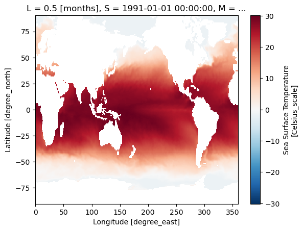
Tip

pcolormesh method generates a map plot that reflects the true value at each grid point. contour or contourf methods, on the other hand, generate interpolated map plots. It is a personal choice and sometimes depends on the purpose of the plots. However, the pcolormesh method would be the best way to represent the actual value in the dataset and not the interpolated result.

Calculate the ensemble mean climatology

The climatology of the ensemble mean is determined based on two steps.

• Calculate the ensemble mean of all ensemble members in each specific model (in our example GFDL-SPEAR)

• Calculate the monthly climatology from the ensemble mean.

The calculation is based on the hindcast. If there is more than one model, each model will have its ensemble mean climatology.

Important

For demonstration in this notebook, the climatology period is only based on one year which does not make sense scientifically but this allows users to quickly play around with the data. For the scientific purpose, the hindcast should at least has 30 years of data to calculate a more meaningful climatology.

# one year of data for climatology (demo purpose only)
start_year = 2020
end_year = 2020

The code loop through different models (in this case GFDL-SPEAR only), downloads the desired period, calculate the ensemble mean, and calculate the climatology of the ensemble mean.

for nmodel,model in enumerate(model_list):
    print('-------------')
    print(model)
    print('-------------')

    # crop data to the desired period
    with ProgressBar():
        da_model = dict_model_hindcast[model].sst.where(
            (dict_model_hindcast[model]['S.year']>=start_year)&
            (dict_model_hindcast[model]['S.year']<=end_year),
            drop=True).compute()
    
    # calculate ensemble mean
    print('calculate ensemble mean')
    da_ensmean = da_model.mean(dim='M')

    # calculate ensemble mean climatology
    print('calculate climatology')
    da_ensmean_climo = da_ensmean.groupby('S.month').mean(dim='S')

-------------
GFDL-SPEAR
-------------

[                                        ] | 0% Completed | 198.94 us

[                                        ] | 0% Completed | 116.47 ms

[                                        ] | 0% Completed | 246.15 ms

[                                        ] | 0% Completed | 356.46 ms

[                                        ] | 0% Completed | 463.99 ms

[                                        ] | 0% Completed | 568.88 ms

[                                        ] | 0% Completed | 669.53 ms

[                                        ] | 0% Completed | 770.31 ms

[                                        ] | 0% Completed | 871.14 ms

[                                        ] | 1% Completed | 971.72 ms

[                                        ] | 1% Completed | 1.08 s

[                                        ] | 2% Completed | 1.19 s

[#                                       ] | 3% Completed | 1.30 s

[#                                       ] | 4% Completed | 1.41 s

[#                                       ] | 4% Completed | 1.53 s

[##                                      ] | 6% Completed | 1.65 s

[##                                      ] | 6% Completed | 1.76 s

[##                                      ] | 6% Completed | 1.86 s

[##                                      ] | 7% Completed | 1.96 s

[###                                     ] | 8% Completed | 2.06 s

[###                                     ] | 8% Completed | 2.17 s

[###                                     ] | 9% Completed | 2.28 s

[####                                    ] | 10% Completed | 2.39 s

[####                                    ] | 11% Completed | 2.49 s

[####                                    ] | 11% Completed | 2.59 s

[#####                                   ] | 12% Completed | 2.70 s

[#####                                   ] | 13% Completed | 2.80 s

[#####                                   ] | 13% Completed | 2.90 s

[#####                                   ] | 14% Completed | 3.01 s

[#####                                   ] | 14% Completed | 3.12 s

[######                                  ] | 15% Completed | 3.23 s

[######                                  ] | 16% Completed | 3.34 s

[######                                  ] | 17% Completed | 3.45 s

[#######                                 ] | 18% Completed | 3.55 s

[#######                                 ] | 19% Completed | 3.66 s

[#######                                 ] | 19% Completed | 3.79 s

[########                                ] | 20% Completed | 3.92 s

[########                                ] | 21% Completed | 4.03 s

[########                                ] | 22% Completed | 4.13 s

[########                                ] | 22% Completed | 4.23 s

[########                                ] | 22% Completed | 4.34 s

[########                                ] | 22% Completed | 4.44 s

[########                                ] | 22% Completed | 4.54 s

[########                                ] | 22% Completed | 4.64 s

[########                                ] | 22% Completed | 4.74 s

[########                                ] | 22% Completed | 4.84 s

[########                                ] | 22% Completed | 4.94 s

[########                                ] | 22% Completed | 5.04 s

[########                                ] | 22% Completed | 5.15 s

[########                                ] | 22% Completed | 5.25 s

[########                                ] | 22% Completed | 5.35 s

[########                                ] | 22% Completed | 5.45 s

[########                                ] | 22% Completed | 5.55 s

[########                                ] | 22% Completed | 5.65 s

[########                                ] | 22% Completed | 5.75 s

[########                                ] | 22% Completed | 5.86 s

[########                                ] | 22% Completed | 5.96 s

[########                                ] | 22% Completed | 6.06 s

[########                                ] | 22% Completed | 6.16 s

[########                                ] | 22% Completed | 6.26 s

[########                                ] | 22% Completed | 6.36 s

[########                                ] | 22% Completed | 6.46 s

[########                                ] | 22% Completed | 6.57 s

[########                                ] | 22% Completed | 6.67 s

[########                                ] | 22% Completed | 6.77 s

[########                                ] | 22% Completed | 6.87 s

[########                                ] | 22% Completed | 6.98 s

[########                                ] | 22% Completed | 7.08 s

[########                                ] | 22% Completed | 7.18 s

[########                                ] | 22% Completed | 7.28 s

[########                                ] | 22% Completed | 7.38 s

[#########                               ] | 22% Completed | 7.49 s

[#########                               ] | 23% Completed | 7.60 s

[#########                               ] | 23% Completed | 7.70 s

[#########                               ] | 24% Completed | 7.80 s

[##########                              ] | 25% Completed | 7.90 s

[##########                              ] | 26% Completed | 8.01 s

[##########                              ] | 26% Completed | 8.11 s

[###########                             ] | 27% Completed | 8.22 s

[###########                             ] | 28% Completed | 8.32 s

[###########                             ] | 29% Completed | 8.43 s

[###########                             ] | 29% Completed | 8.53 s

[############                            ] | 30% Completed | 8.63 s

[############                            ] | 31% Completed | 8.74 s

[############                            ] | 31% Completed | 8.84 s

[############                            ] | 31% Completed | 8.94 s

[############                            ] | 31% Completed | 9.04 s

[############                            ] | 32% Completed | 9.14 s

[#############                           ] | 32% Completed | 9.25 s

[#############                           ] | 33% Completed | 9.35 s

[#############                           ] | 33% Completed | 9.45 s

[#############                           ] | 33% Completed | 9.55 s

[#############                           ] | 33% Completed | 9.65 s

[#############                           ] | 34% Completed | 9.75 s

[#############                           ] | 34% Completed | 9.86 s

[##############                          ] | 35% Completed | 9.96 s

[##############                          ] | 36% Completed | 10.07 s

[###############                         ] | 37% Completed | 10.18 s

[###############                         ] | 38% Completed | 10.29 s

[###############                         ] | 39% Completed | 10.39 s

[################                        ] | 40% Completed | 10.49 s

[################                        ] | 40% Completed | 10.59 s

[################                        ] | 40% Completed | 10.70 s

[################                        ] | 41% Completed | 10.80 s

[################                        ] | 41% Completed | 10.90 s

[#################                       ] | 43% Completed | 11.01 s

[#################                       ] | 44% Completed | 11.12 s

[#################                       ] | 44% Completed | 11.23 s

[#################                       ] | 44% Completed | 11.33 s

[#################                       ] | 44% Completed | 11.43 s

[#################                       ] | 44% Completed | 11.53 s

[#################                       ] | 44% Completed | 11.64 s

[#################                       ] | 44% Completed | 11.74 s

[#################                       ] | 44% Completed | 11.84 s

[#################                       ] | 44% Completed | 11.94 s

[#################                       ] | 44% Completed | 12.04 s

[#################                       ] | 44% Completed | 12.14 s

[#################                       ] | 44% Completed | 12.24 s

[#################                       ] | 44% Completed | 12.34 s

[#################                       ] | 44% Completed | 12.44 s

[#################                       ] | 44% Completed | 12.54 s

[#################                       ] | 44% Completed | 12.64 s

[#################                       ] | 44% Completed | 12.75 s

[#################                       ] | 44% Completed | 12.85 s

[#################                       ] | 44% Completed | 12.95 s

[#################                       ] | 44% Completed | 13.05 s

[#################                       ] | 44% Completed | 13.15 s

[#################                       ] | 44% Completed | 13.25 s

[#################                       ] | 44% Completed | 13.35 s

[#################                       ] | 44% Completed | 13.46 s

[#################                       ] | 44% Completed | 13.56 s

[#################                       ] | 44% Completed | 13.66 s

[#################                       ] | 44% Completed | 13.76 s

[#################                       ] | 44% Completed | 13.86 s

[#################                       ] | 44% Completed | 13.96 s

[#################                       ] | 44% Completed | 14.06 s

[#################                       ] | 44% Completed | 14.16 s

[##################                      ] | 45% Completed | 14.26 s

[##################                      ] | 45% Completed | 14.37 s

[##################                      ] | 45% Completed | 14.47 s

[##################                      ] | 46% Completed | 14.57 s

[##################                      ] | 46% Completed | 14.68 s

[##################                      ] | 47% Completed | 14.78 s

[###################                     ] | 47% Completed | 14.88 s

[###################                     ] | 48% Completed | 14.98 s

[###################                     ] | 49% Completed | 15.09 s

[####################                    ] | 50% Completed | 15.20 s

[####################                    ] | 51% Completed | 15.30 s

[####################                    ] | 52% Completed | 15.40 s

[####################                    ] | 52% Completed | 15.50 s

[#####################                   ] | 52% Completed | 15.60 s

[#####################                   ] | 52% Completed | 15.70 s

[#####################                   ] | 53% Completed | 15.80 s

[#####################                   ] | 54% Completed | 15.91 s

[######################                  ] | 55% Completed | 16.01 s

[######################                  ] | 55% Completed | 16.11 s

[######################                  ] | 56% Completed | 16.22 s

[#######################                 ] | 57% Completed | 16.32 s

[#######################                 ] | 58% Completed | 16.43 s

[#######################                 ] | 59% Completed | 16.54 s

[#######################                 ] | 59% Completed | 16.64 s

[#######################                 ] | 59% Completed | 16.74 s

[#######################                 ] | 59% Completed | 16.84 s

[#######################                 ] | 59% Completed | 16.94 s

[########################                ] | 60% Completed | 17.05 s

[########################                ] | 60% Completed | 17.15 s

[########################                ] | 60% Completed | 17.25 s

[########################                ] | 60% Completed | 17.35 s

[########################                ] | 60% Completed | 17.45 s

[########################                ] | 60% Completed | 17.55 s

[########################                ] | 61% Completed | 17.65 s

[########################                ] | 61% Completed | 17.75 s

[########################                ] | 62% Completed | 17.86 s

[########################                ] | 62% Completed | 17.96 s

[#########################               ] | 63% Completed | 18.06 s

[#########################               ] | 64% Completed | 18.18 s

[##########################              ] | 65% Completed | 18.28 s

[##########################              ] | 66% Completed | 18.39 s

[##########################              ] | 66% Completed | 18.49 s

[##########################              ] | 66% Completed | 18.59 s

[##########################              ] | 66% Completed | 18.69 s

[##########################              ] | 66% Completed | 18.79 s

[##########################              ] | 66% Completed | 18.90 s

[##########################              ] | 67% Completed | 19.00 s

[##########################              ] | 67% Completed | 19.10 s

[##########################              ] | 67% Completed | 19.20 s

[##########################              ] | 67% Completed | 19.30 s

[##########################              ] | 67% Completed | 19.40 s

[##########################              ] | 67% Completed | 19.50 s

[##########################              ] | 67% Completed | 19.60 s

[##########################              ] | 67% Completed | 19.70 s

[##########################              ] | 67% Completed | 19.81 s

[##########################              ] | 67% Completed | 19.91 s

[##########################              ] | 67% Completed | 20.01 s

[##########################              ] | 67% Completed | 20.11 s

[##########################              ] | 67% Completed | 20.21 s

[##########################              ] | 67% Completed | 20.31 s

[##########################              ] | 67% Completed | 20.41 s

[##########################              ] | 67% Completed | 20.51 s

[##########################              ] | 67% Completed | 20.62 s

[##########################              ] | 67% Completed | 20.72 s

[##########################              ] | 67% Completed | 20.82 s

[##########################              ] | 67% Completed | 20.92 s

[##########################              ] | 67% Completed | 21.02 s

[##########################              ] | 67% Completed | 21.13 s

[##########################              ] | 67% Completed | 21.23 s

[##########################              ] | 67% Completed | 21.33 s

[##########################              ] | 67% Completed | 21.43 s

[##########################              ] | 67% Completed | 21.53 s

[##########################              ] | 67% Completed | 21.63 s

[###########################             ] | 67% Completed | 21.86 s

[###########################             ] | 68% Completed | 21.97 s

[###########################             ] | 69% Completed | 22.08 s

[############################            ] | 70% Completed | 22.18 s

[############################            ] | 71% Completed | 22.29 s

[############################            ] | 71% Completed | 22.39 s

[############################            ] | 71% Completed | 22.49 s

[############################            ] | 72% Completed | 22.59 s

[############################            ] | 72% Completed | 22.70 s

[#############################           ] | 72% Completed | 22.80 s

[#############################           ] | 73% Completed | 22.90 s

[#############################           ] | 74% Completed | 23.02 s

[##############################          ] | 75% Completed | 23.12 s

[##############################          ] | 76% Completed | 23.23 s

[##############################          ] | 77% Completed | 23.34 s

[###############################         ] | 77% Completed | 23.45 s

[###############################         ] | 78% Completed | 23.56 s

[###############################         ] | 78% Completed | 23.66 s

[###############################         ] | 79% Completed | 23.76 s

[################################        ] | 80% Completed | 23.86 s

[################################        ] | 81% Completed | 23.97 s

[################################        ] | 82% Completed | 24.08 s

[#################################       ] | 83% Completed | 24.19 s

[#################################       ] | 83% Completed | 24.29 s

[#################################       ] | 84% Completed | 24.40 s

[#################################       ] | 84% Completed | 24.50 s

[##################################      ] | 85% Completed | 24.60 s

[##################################      ] | 86% Completed | 24.70 s

[##################################      ] | 86% Completed | 24.81 s

[##################################      ] | 86% Completed | 24.91 s

[##################################      ] | 86% Completed | 25.01 s

[##################################      ] | 87% Completed | 25.11 s

[###################################     ] | 88% Completed | 25.21 s

[###################################     ] | 88% Completed | 25.31 s

[###################################     ] | 88% Completed | 25.41 s

[###################################     ] | 88% Completed | 25.51 s

[###################################     ] | 89% Completed | 25.62 s

[###################################     ] | 89% Completed | 25.72 s

[###################################     ] | 89% Completed | 25.82 s

[###################################     ] | 89% Completed | 25.92 s

[###################################     ] | 89% Completed | 26.02 s

[###################################     ] | 89% Completed | 26.12 s

[###################################     ] | 89% Completed | 26.23 s

[###################################     ] | 89% Completed | 26.33 s

[###################################     ] | 89% Completed | 26.43 s

[###################################     ] | 89% Completed | 26.53 s

[###################################     ] | 89% Completed | 26.63 s

[###################################     ] | 89% Completed | 26.73 s

[###################################     ] | 89% Completed | 26.83 s

[###################################     ] | 89% Completed | 26.93 s

[###################################     ] | 89% Completed | 27.03 s

[###################################     ] | 89% Completed | 27.14 s

[###################################     ] | 89% Completed | 27.24 s

[###################################     ] | 89% Completed | 27.34 s

[###################################     ] | 89% Completed | 27.44 s

[###################################     ] | 89% Completed | 27.54 s

[###################################     ] | 89% Completed | 27.64 s

[###################################     ] | 89% Completed | 27.74 s

[####################################    ] | 90% Completed | 27.84 s

[####################################    ] | 91% Completed | 27.95 s

[####################################    ] | 91% Completed | 28.05 s

[####################################    ] | 92% Completed | 28.16 s

[####################################    ] | 92% Completed | 28.26 s

[#####################################   ] | 92% Completed | 28.36 s

[#####################################   ] | 92% Completed | 28.46 s

[#####################################   ] | 92% Completed | 28.56 s

[#####################################   ] | 92% Completed | 28.67 s

[#####################################   ] | 92% Completed | 28.78 s

[#####################################   ] | 92% Completed | 28.88 s

[#####################################   ] | 92% Completed | 28.98 s

[#####################################   ] | 92% Completed | 29.08 s

[#####################################   ] | 92% Completed | 29.19 s

[#####################################   ] | 92% Completed | 29.29 s

[#####################################   ] | 93% Completed | 29.40 s

[#####################################   ] | 93% Completed | 29.50 s

[#####################################   ] | 94% Completed | 29.61 s

[######################################  ] | 95% Completed | 29.71 s

[######################################  ] | 95% Completed | 29.81 s

[######################################  ] | 95% Completed | 29.91 s

[######################################  ] | 96% Completed | 30.01 s

[######################################  ] | 97% Completed | 30.11 s

[####################################### ] | 97% Completed | 30.21 s

[####################################### ] | 98% Completed | 30.31 s

[####################################### ] | 98% Completed | 30.41 s

[####################################### ] | 98% Completed | 30.52 s

[####################################### ] | 98% Completed | 30.62 s

[####################################### ] | 98% Completed | 30.72 s

[####################################### ] | 98% Completed | 30.82 s

[####################################### ] | 98% Completed | 30.92 s

[####################################### ] | 98% Completed | 31.02 s

[####################################### ] | 98% Completed | 31.13 s

[####################################### ] | 98% Completed | 31.23 s

[####################################### ] | 98% Completed | 31.33 s

[####################################### ] | 98% Completed | 31.43 s

[####################################### ] | 98% Completed | 31.53 s

[####################################### ] | 98% Completed | 31.63 s

[####################################### ] | 98% Completed | 31.73 s

[####################################### ] | 98% Completed | 31.83 s

[####################################### ] | 98% Completed | 31.93 s

[####################################### ] | 98% Completed | 32.03 s

[####################################### ] | 98% Completed | 32.13 s

[####################################### ] | 98% Completed | 32.23 s

[####################################### ] | 98% Completed | 32.33 s

[####################################### ] | 98% Completed | 32.43 s

[####################################### ] | 98% Completed | 32.54 s

[####################################### ] | 98% Completed | 32.64 s

[####################################### ] | 98% Completed | 32.74 s

[####################################### ] | 99% Completed | 32.84 s

[####################################### ] | 99% Completed | 32.94 s

[########################################] | 100% Completed | 33.04 s

calculate ensemble mean

calculate climatology

Tip

Only till this point of the code with .compute(), the data is downloaded to the local memory and cropped to our desired period. The ProgressBar() method provided by the dask package gives us a quick way to monitor the progress of the data query in the notebook.

To do a quick peak on the calculated da_ensmean and da_ensmean_climo

da_ensmean

<xarray.DataArray 'sst' (S: 12, L: 12, Y: 181, X: 360)>
array([[[[        nan,         nan,         nan, ...,         nan,
                  nan,         nan],
         [        nan,         nan,         nan, ...,         nan,
                  nan,         nan],
         [        nan,         nan,         nan, ...,         nan,
                  nan,         nan],
         ...,
         [-1.8152167 , -1.7997636 , -1.8374307 , ..., -1.7942959 ,
          -1.8131804 , -1.8267497 ],
         [-1.8465025 , -1.8499216 , -1.8553926 , ..., -1.8044785 ,
          -1.8234142 , -1.8409054 ],
         [        nan,         nan,         nan, ...,         nan,
                  nan,         nan]],

        [[        nan,         nan,         nan, ...,         nan,
                  nan,         nan],
         [        nan,         nan,         nan, ...,         nan,
                  nan,         nan],
         [        nan,         nan,         nan, ...,         nan,
                  nan,         nan],
...
         [-0.40647423, -0.32241496, -0.32639506, ..., -1.2913983 ,
          -1.0387492 , -0.67631894],
         [-0.53427947, -0.25783926, -0.15042621, ..., -1.2976335 ,
          -1.157531  , -0.9127232 ],
         [        nan,         nan,         nan, ...,         nan,
                  nan,         nan]],

        [[        nan,         nan,         nan, ...,         nan,
                  nan,         nan],
         [        nan,         nan,         nan, ...,         nan,
                  nan,         nan],
         [        nan,         nan,         nan, ...,         nan,
                  nan,         nan],
         ...,
         [-1.3329976 , -1.2299353 , -1.227057  , ..., -1.6917287 ,
          -1.6293875 , -1.4921345 ],
         [-1.4859961 , -1.4001585 , -1.3600676 , ..., -1.7011333 ,
          -1.6687951 , -1.5964279 ],
         [        nan,         nan,         nan, ...,         nan,
                  nan,         nan]]]], dtype=float32)
Coordinates:
  * Y        (Y) float32 -90.0 -89.0 -88.0 -87.0 -86.0 ... 87.0 88.0 89.0 90.0
  * L        (L) float32 0.5 1.5 2.5 3.5 4.5 5.5 6.5 7.5 8.5 9.5 10.5 11.5
  * S        (S) object 2020-01-01 00:00:00 ... 2020-12-01 00:00:00
  * X        (X) float32 0.0 1.0 2.0 3.0 4.0 ... 355.0 356.0 357.0 358.0 359.0

xarray.DataArray

'sst'

• S: 12
• L: 12
• Y: 181
• X: 360

• nan nan nan nan nan nan nan nan ... nan nan nan nan nan nan nan nan

  array([[[[        nan,         nan,         nan, ...,         nan,
                    nan,         nan],
           [        nan,         nan,         nan, ...,         nan,
                    nan,         nan],
           [        nan,         nan,         nan, ...,         nan,
                    nan,         nan],
           ...,
           [-1.8152167 , -1.7997636 , -1.8374307 , ..., -1.7942959 ,
            -1.8131804 , -1.8267497 ],
           [-1.8465025 , -1.8499216 , -1.8553926 , ..., -1.8044785 ,
            -1.8234142 , -1.8409054 ],
           [        nan,         nan,         nan, ...,         nan,
                    nan,         nan]],
  
          [[        nan,         nan,         nan, ...,         nan,
                    nan,         nan],
           [        nan,         nan,         nan, ...,         nan,
                    nan,         nan],
           [        nan,         nan,         nan, ...,         nan,
                    nan,         nan],
  ...
           [-0.40647423, -0.32241496, -0.32639506, ..., -1.2913983 ,
            -1.0387492 , -0.67631894],
           [-0.53427947, -0.25783926, -0.15042621, ..., -1.2976335 ,
            -1.157531  , -0.9127232 ],
           [        nan,         nan,         nan, ...,         nan,
                    nan,         nan]],
  
          [[        nan,         nan,         nan, ...,         nan,
                    nan,         nan],
           [        nan,         nan,         nan, ...,         nan,
                    nan,         nan],
           [        nan,         nan,         nan, ...,         nan,
                    nan,         nan],
           ...,
           [-1.3329976 , -1.2299353 , -1.227057  , ..., -1.6917287 ,
            -1.6293875 , -1.4921345 ],
           [-1.4859961 , -1.4001585 , -1.3600676 , ..., -1.7011333 ,
            -1.6687951 , -1.5964279 ],
           [        nan,         nan,         nan, ...,         nan,
                    nan,         nan]]]], dtype=float32)

• Coordinates: (4)
  • Y
    (Y)
    float32
    -90.0 -89.0 -88.0 ... 89.0 90.0

    standard_name :

    latitude

    long_name :

    Latitude

    pointwidth :

    1.0

    gridtype :

    0

    units :

    degree_north

    array([-90., -89., -88., -87., -86., -85., -84., -83., -82., -81., -80., -79.,
           -78., -77., -76., -75., -74., -73., -72., -71., -70., -69., -68., -67.,
           -66., -65., -64., -63., -62., -61., -60., -59., -58., -57., -56., -55.,
           -54., -53., -52., -51., -50., -49., -48., -47., -46., -45., -44., -43.,
           -42., -41., -40., -39., -38., -37., -36., -35., -34., -33., -32., -31.,
           -30., -29., -28., -27., -26., -25., -24., -23., -22., -21., -20., -19.,
           -18., -17., -16., -15., -14., -13., -12., -11., -10.,  -9.,  -8.,  -7.,
            -6.,  -5.,  -4.,  -3.,  -2.,  -1.,   0.,   1.,   2.,   3.,   4.,   5.,
             6.,   7.,   8.,   9.,  10.,  11.,  12.,  13.,  14.,  15.,  16.,  17.,
            18.,  19.,  20.,  21.,  22.,  23.,  24.,  25.,  26.,  27.,  28.,  29.,
            30.,  31.,  32.,  33.,  34.,  35.,  36.,  37.,  38.,  39.,  40.,  41.,
            42.,  43.,  44.,  45.,  46.,  47.,  48.,  49.,  50.,  51.,  52.,  53.,
            54.,  55.,  56.,  57.,  58.,  59.,  60.,  61.,  62.,  63.,  64.,  65.,
            66.,  67.,  68.,  69.,  70.,  71.,  72.,  73.,  74.,  75.,  76.,  77.,
            78.,  79.,  80.,  81.,  82.,  83.,  84.,  85.,  86.,  87.,  88.,  89.,
            90.], dtype=float32)

  • L
    (L)
    float32
    0.5 1.5 2.5 3.5 ... 9.5 10.5 11.5

    standard_name :

    forecast_period

    long_name :

    Lead

    pointwidth :

    1.0

    gridtype :

    0

    units :

    months

    array([ 0.5,  1.5,  2.5,  3.5,  4.5,  5.5,  6.5,  7.5,  8.5,  9.5, 10.5, 11.5],
          dtype=float32)

  • S
    (S)
    object
    2020-01-01 00:00:00 ... 2020-12-...

    array([cftime.Datetime360Day(2020, 1, 1, 0, 0, 0, 0, has_year_zero=True),
           cftime.Datetime360Day(2020, 2, 1, 0, 0, 0, 0, has_year_zero=True),
           cftime.Datetime360Day(2020, 3, 1, 0, 0, 0, 0, has_year_zero=True),
           cftime.Datetime360Day(2020, 4, 1, 0, 0, 0, 0, has_year_zero=True),
           cftime.Datetime360Day(2020, 5, 1, 0, 0, 0, 0, has_year_zero=True),
           cftime.Datetime360Day(2020, 6, 1, 0, 0, 0, 0, has_year_zero=True),
           cftime.Datetime360Day(2020, 7, 1, 0, 0, 0, 0, has_year_zero=True),
           cftime.Datetime360Day(2020, 8, 1, 0, 0, 0, 0, has_year_zero=True),
           cftime.Datetime360Day(2020, 9, 1, 0, 0, 0, 0, has_year_zero=True),
           cftime.Datetime360Day(2020, 10, 1, 0, 0, 0, 0, has_year_zero=True),
           cftime.Datetime360Day(2020, 11, 1, 0, 0, 0, 0, has_year_zero=True),
           cftime.Datetime360Day(2020, 12, 1, 0, 0, 0, 0, has_year_zero=True)],
          dtype=object)

  • X
    (X)
    float32
    0.0 1.0 2.0 ... 357.0 358.0 359.0

    standard_name :

    longitude

    long_name :

    Longitude

    pointwidth :

    1.0

    gridtype :

    1

    units :

    degree_east

    array([  0.,   1.,   2., ..., 357., 358., 359.], dtype=float32)

• Indexes: (4)
  • Y
    PandasIndex

    PandasIndex(Float64Index([-90.0, -89.0, -88.0, -87.0, -86.0, -85.0, -84.0, -83.0, -82.0,
                  -81.0,
                  ...
                   81.0,  82.0,  83.0,  84.0,  85.0,  86.0,  87.0,  88.0,  89.0,
                   90.0],
                 dtype='float64', name='Y', length=181))

  • L
    PandasIndex

    PandasIndex(Float64Index([0.5, 1.5, 2.5, 3.5, 4.5, 5.5, 6.5, 7.5, 8.5, 9.5, 10.5, 11.5], dtype='float64', name='L'))

  • S
    PandasIndex

    PandasIndex(CFTimeIndex([2020-01-01 00:00:00, 2020-02-01 00:00:00, 2020-03-01 00:00:00,
                 2020-04-01 00:00:00, 2020-05-01 00:00:00, 2020-06-01 00:00:00,
                 2020-07-01 00:00:00, 2020-08-01 00:00:00, 2020-09-01 00:00:00,
                 2020-10-01 00:00:00, 2020-11-01 00:00:00, 2020-12-01 00:00:00],
                dtype='object', length=12, calendar='360_day', freq='MS'))

  • X
    PandasIndex

    PandasIndex(Float64Index([  0.0,   1.0,   2.0,   3.0,   4.0,   5.0,   6.0,   7.0,   8.0,
                    9.0,
                  ...
                  350.0, 351.0, 352.0, 353.0, 354.0, 355.0, 356.0, 357.0, 358.0,
                  359.0],
                 dtype='float64', name='X', length=360))

• Attributes: (0)

da_ensmean_climo

<xarray.DataArray 'sst' (month: 12, L: 12, Y: 181, X: 360)>
array([[[[        nan,         nan,         nan, ...,         nan,
                  nan,         nan],
         [        nan,         nan,         nan, ...,         nan,
                  nan,         nan],
         [        nan,         nan,         nan, ...,         nan,
                  nan,         nan],
         ...,
         [-1.8152167 , -1.7997636 , -1.8374307 , ..., -1.7942959 ,
          -1.8131804 , -1.8267497 ],
         [-1.8465025 , -1.8499216 , -1.8553926 , ..., -1.8044785 ,
          -1.8234142 , -1.8409054 ],
         [        nan,         nan,         nan, ...,         nan,
                  nan,         nan]],

        [[        nan,         nan,         nan, ...,         nan,
                  nan,         nan],
         [        nan,         nan,         nan, ...,         nan,
                  nan,         nan],
         [        nan,         nan,         nan, ...,         nan,
                  nan,         nan],
...
         [-0.40647423, -0.32241496, -0.32639506, ..., -1.2913983 ,
          -1.0387492 , -0.67631894],
         [-0.53427947, -0.25783926, -0.15042621, ..., -1.2976335 ,
          -1.157531  , -0.9127232 ],
         [        nan,         nan,         nan, ...,         nan,
                  nan,         nan]],

        [[        nan,         nan,         nan, ...,         nan,
                  nan,         nan],
         [        nan,         nan,         nan, ...,         nan,
                  nan,         nan],
         [        nan,         nan,         nan, ...,         nan,
                  nan,         nan],
         ...,
         [-1.3329976 , -1.2299353 , -1.227057  , ..., -1.6917287 ,
          -1.6293875 , -1.4921345 ],
         [-1.4859961 , -1.4001585 , -1.3600676 , ..., -1.7011333 ,
          -1.6687951 , -1.5964279 ],
         [        nan,         nan,         nan, ...,         nan,
                  nan,         nan]]]], dtype=float32)
Coordinates:
  * Y        (Y) float32 -90.0 -89.0 -88.0 -87.0 -86.0 ... 87.0 88.0 89.0 90.0
  * L        (L) float32 0.5 1.5 2.5 3.5 4.5 5.5 6.5 7.5 8.5 9.5 10.5 11.5
  * X        (X) float32 0.0 1.0 2.0 3.0 4.0 ... 355.0 356.0 357.0 358.0 359.0
  * month    (month) int64 1 2 3 4 5 6 7 8 9 10 11 12

xarray.DataArray

'sst'

• month: 12
• L: 12
• Y: 181
• X: 360

• nan nan nan nan nan nan nan nan ... nan nan nan nan nan nan nan nan

  array([[[[        nan,         nan,         nan, ...,         nan,
                    nan,         nan],
           [        nan,         nan,         nan, ...,         nan,
                    nan,         nan],
           [        nan,         nan,         nan, ...,         nan,
                    nan,         nan],
           ...,
           [-1.8152167 , -1.7997636 , -1.8374307 , ..., -1.7942959 ,
            -1.8131804 , -1.8267497 ],
           [-1.8465025 , -1.8499216 , -1.8553926 , ..., -1.8044785 ,
            -1.8234142 , -1.8409054 ],
           [        nan,         nan,         nan, ...,         nan,
                    nan,         nan]],
  
          [[        nan,         nan,         nan, ...,         nan,
                    nan,         nan],
           [        nan,         nan,         nan, ...,         nan,
                    nan,         nan],
           [        nan,         nan,         nan, ...,         nan,
                    nan,         nan],
  ...
           [-0.40647423, -0.32241496, -0.32639506, ..., -1.2913983 ,
            -1.0387492 , -0.67631894],
           [-0.53427947, -0.25783926, -0.15042621, ..., -1.2976335 ,
            -1.157531  , -0.9127232 ],
           [        nan,         nan,         nan, ...,         nan,
                    nan,         nan]],
  
          [[        nan,         nan,         nan, ...,         nan,
                    nan,         nan],
           [        nan,         nan,         nan, ...,         nan,
                    nan,         nan],
           [        nan,         nan,         nan, ...,         nan,
                    nan,         nan],
           ...,
           [-1.3329976 , -1.2299353 , -1.227057  , ..., -1.6917287 ,
            -1.6293875 , -1.4921345 ],
           [-1.4859961 , -1.4001585 , -1.3600676 , ..., -1.7011333 ,
            -1.6687951 , -1.5964279 ],
           [        nan,         nan,         nan, ...,         nan,
                    nan,         nan]]]], dtype=float32)

• Coordinates: (4)
  • Y
    (Y)
    float32
    -90.0 -89.0 -88.0 ... 89.0 90.0

    standard_name :

    latitude

    long_name :

    Latitude

    pointwidth :

    1.0

    gridtype :

    0

    units :

    degree_north

    array([-90., -89., -88., -87., -86., -85., -84., -83., -82., -81., -80., -79.,
           -78., -77., -76., -75., -74., -73., -72., -71., -70., -69., -68., -67.,
           -66., -65., -64., -63., -62., -61., -60., -59., -58., -57., -56., -55.,
           -54., -53., -52., -51., -50., -49., -48., -47., -46., -45., -44., -43.,
           -42., -41., -40., -39., -38., -37., -36., -35., -34., -33., -32., -31.,
           -30., -29., -28., -27., -26., -25., -24., -23., -22., -21., -20., -19.,
           -18., -17., -16., -15., -14., -13., -12., -11., -10.,  -9.,  -8.,  -7.,
            -6.,  -5.,  -4.,  -3.,  -2.,  -1.,   0.,   1.,   2.,   3.,   4.,   5.,
             6.,   7.,   8.,   9.,  10.,  11.,  12.,  13.,  14.,  15.,  16.,  17.,
            18.,  19.,  20.,  21.,  22.,  23.,  24.,  25.,  26.,  27.,  28.,  29.,
            30.,  31.,  32.,  33.,  34.,  35.,  36.,  37.,  38.,  39.,  40.,  41.,
            42.,  43.,  44.,  45.,  46.,  47.,  48.,  49.,  50.,  51.,  52.,  53.,
            54.,  55.,  56.,  57.,  58.,  59.,  60.,  61.,  62.,  63.,  64.,  65.,
            66.,  67.,  68.,  69.,  70.,  71.,  72.,  73.,  74.,  75.,  76.,  77.,
            78.,  79.,  80.,  81.,  82.,  83.,  84.,  85.,  86.,  87.,  88.,  89.,
            90.], dtype=float32)

  • L
    (L)
    float32
    0.5 1.5 2.5 3.5 ... 9.5 10.5 11.5

    standard_name :

    forecast_period

    long_name :

    Lead

    pointwidth :

    1.0

    gridtype :

    0

    units :

    months

    array([ 0.5,  1.5,  2.5,  3.5,  4.5,  5.5,  6.5,  7.5,  8.5,  9.5, 10.5, 11.5],
          dtype=float32)

  • X
    (X)
    float32
    0.0 1.0 2.0 ... 357.0 358.0 359.0

    standard_name :

    longitude

    long_name :

    Longitude

    pointwidth :

    1.0

    gridtype :

    1

    units :

    degree_east

    array([  0.,   1.,   2., ..., 357., 358., 359.], dtype=float32)

  • month
    (month)
    int64
    1 2 3 4 5 6 7 8 9 10 11 12

    array([ 1,  2,  3,  4,  5,  6,  7,  8,  9, 10, 11, 12])

• Indexes: (4)
  • Y
    PandasIndex

    PandasIndex(Float64Index([-90.0, -89.0, -88.0, -87.0, -86.0, -85.0, -84.0, -83.0, -82.0,
                  -81.0,
                  ...
                   81.0,  82.0,  83.0,  84.0,  85.0,  86.0,  87.0,  88.0,  89.0,
                   90.0],
                 dtype='float64', name='Y', length=181))

  • L
    PandasIndex

    PandasIndex(Float64Index([0.5, 1.5, 2.5, 3.5, 4.5, 5.5, 6.5, 7.5, 8.5, 9.5, 10.5, 11.5], dtype='float64', name='L'))

  • X
    PandasIndex

    PandasIndex(Float64Index([  0.0,   1.0,   2.0,   3.0,   4.0,   5.0,   6.0,   7.0,   8.0,
                    9.0,
                  ...
                  350.0, 351.0, 352.0, 353.0, 354.0, 355.0, 356.0, 357.0, 358.0,
                  359.0],
                 dtype='float64', name='X', length=360))

  • month
    PandasIndex

    PandasIndex(Int64Index([1, 2, 3, 4, 5, 6, 7, 8, 9, 10, 11, 12], dtype='int64', name='month'))

• Attributes: (0)

We can see the da_ensmean has one dimension less than the original dataset due to the ensemble member dimension M being averaged. The da_ensmean_climo, on the other hand, is grouped by the month of the year.

Calculate the threshold

The monthly threshold is based on the hindcast SST anomaly with a three-month window (initial months) for each initial time (centered month) and associated lead time.

Example:

The January (initial month) threshold of lead time = 0.5,1.5,2.5,… month is determined by all ensemble members with December, January, and February SST anomaly at lead time = 0.5,1.5,2.5,… month, respectively.

Define functions

The function below performs the three-month window on all initial months to find the corresponding monthly threshold at each lead time.

def nmme_3mon_quantile(da_data, mhw_threshold=90.):
    """
    This function is designed for calculating the nmme 
    marine heat wave threshold.
    
    The threshold is calculated using a 3 month window
    to identified the X quantile value for each month.

    Parameters
    ----------
    da_data : xr.DataArray 
        For marine heat wave calculation, it should be the sst DataArray. 
        Since this function is designed for NMME model. The DataArray need 
        to be in the format of NMME model output.
    mhw_threshold : float
        the X quantile one wants to calculate. 

    Returns
    -------
    da_data_quantile : xr.DataArray
        The xr.DataArray for the quantile 

    Raises
    ------

    """
    
    da_data_quantile = xr.DataArray(coords={'X':da_data.X,
                                            'Y':da_data.Y,
                                            'month':np.arange(1,13),
                                            'L':da_data.L},
                                    dims = ['month','L','Y','X'])

    for i in range(1,13):
        print(f"calculate month{i} threshold")
        if i == 1:
            mon_range = [12,1,2]
        elif i == 12 :
            mon_range = [11,12,1]
        else:
            mon_range = [i-1,i,i+1]

        da_data_quantile[i-1,:,:,:] = (da_data
                                 .where((da_data['S.month'] == mon_range[0])|
                                        (da_data['S.month'] == mon_range[1])|
                                        (da_data['S.month'] == mon_range[2]),drop=True)
                                 .stack(allens=('S','M'))
                                 .quantile(mhw_threshold*0.01, dim = 'allens', method='linear',skipna = True))

    return da_data_quantile
    


            

With the function defined, we just need to calculate the SST anomaly in hindcast. There are different methods to determine the quantile. For xarray.quantile method (based on numpy.quantile), one can choose the desired method based on NumPy documentation.

print('calculating anomaly from hindcast')
da_anom = (da_model.groupby('S.month') - da_ensmean_climo)

ds_mhw_threshold = xr.Dataset()

mhw_threshold = [90]
for m in mhw_threshold:

    print(f'calculating threshold {m}')
    da_threshold = nmme_3mon_quantile(da_anom, mhw_threshold=m)
    ds_mhw_threshold[f'threshold_{m}'] = da_threshold

calculating anomaly from hindcast

calculating threshold 90
calculate month1 threshold

calculate month2 threshold

calculate month3 threshold

calculate month4 threshold

calculate month5 threshold

calculate month6 threshold

calculate month7 threshold

calculate month8 threshold

calculate month9 threshold

calculate month10 threshold

calculate month11 threshold

calculate month12 threshold

Warning

The function nmme_3mon_quantile is the most time-consuming part of the whole calculation. It should have a more optimal way to speed up the process. However, this is currently (at the time of creating this notebook) our best solution.

The resulting threshold structure would look like below

da_threshold

<xarray.DataArray (month: 12, L: 12, Y: 181, X: 360)>
array([[[[       nan,        nan,        nan, ...,        nan,
                 nan,        nan],
         [       nan,        nan,        nan, ...,        nan,
                 nan,        nan],
         [       nan,        nan,        nan, ...,        nan,
                 nan,        nan],
         ...,
         [0.03974178, 0.03800244, 0.0391201 , ..., 0.02901187,
          0.02458122, 0.02564578],
         [0.02360184, 0.02258537, 0.02060158, ..., 0.02521191,
          0.02393916, 0.02910042],
         [       nan,        nan,        nan, ...,        nan,
                 nan,        nan]],

        [[       nan,        nan,        nan, ...,        nan,
                 nan,        nan],
         [       nan,        nan,        nan, ...,        nan,
                 nan,        nan],
         [       nan,        nan,        nan, ...,        nan,
                 nan,        nan],
...
         [0.72357243, 0.6991505 , 0.60478079, ..., 0.4973405 ,
          0.57291734, 0.64648652],
         [0.71915537, 0.69076586, 0.86227494, ..., 0.52292567,
          0.60902071, 0.7330662 ],
         [       nan,        nan,        nan, ...,        nan,
                 nan,        nan]],

        [[       nan,        nan,        nan, ...,        nan,
                 nan,        nan],
         [       nan,        nan,        nan, ...,        nan,
                 nan,        nan],
         [       nan,        nan,        nan, ...,        nan,
                 nan,        nan],
         ...,
         [0.48410219, 0.40909404, 0.44498792, ..., 0.18629833,
          0.25511676, 0.40680373],
         [0.58163875, 0.57490486, 0.68392879, ..., 0.13991448,
          0.22305867, 0.47826964],
         [       nan,        nan,        nan, ...,        nan,
                 nan,        nan]]]])
Coordinates:
  * X        (X) float32 0.0 1.0 2.0 3.0 4.0 ... 355.0 356.0 357.0 358.0 359.0
  * Y        (Y) float32 -90.0 -89.0 -88.0 -87.0 -86.0 ... 87.0 88.0 89.0 90.0
  * month    (month) int64 1 2 3 4 5 6 7 8 9 10 11 12
  * L        (L) float32 0.5 1.5 2.5 3.5 4.5 5.5 6.5 7.5 8.5 9.5 10.5 11.5

xarray.DataArray

• month: 12
• L: 12
• Y: 181
• X: 360

• nan nan nan nan nan nan nan nan ... nan nan nan nan nan nan nan nan

  array([[[[       nan,        nan,        nan, ...,        nan,
                   nan,        nan],
           [       nan,        nan,        nan, ...,        nan,
                   nan,        nan],
           [       nan,        nan,        nan, ...,        nan,
                   nan,        nan],
           ...,
           [0.03974178, 0.03800244, 0.0391201 , ..., 0.02901187,
            0.02458122, 0.02564578],
           [0.02360184, 0.02258537, 0.02060158, ..., 0.02521191,
            0.02393916, 0.02910042],
           [       nan,        nan,        nan, ...,        nan,
                   nan,        nan]],
  
          [[       nan,        nan,        nan, ...,        nan,
                   nan,        nan],
           [       nan,        nan,        nan, ...,        nan,
                   nan,        nan],
           [       nan,        nan,        nan, ...,        nan,
                   nan,        nan],
  ...
           [0.72357243, 0.6991505 , 0.60478079, ..., 0.4973405 ,
            0.57291734, 0.64648652],
           [0.71915537, 0.69076586, 0.86227494, ..., 0.52292567,
            0.60902071, 0.7330662 ],
           [       nan,        nan,        nan, ...,        nan,
                   nan,        nan]],
  
          [[       nan,        nan,        nan, ...,        nan,
                   nan,        nan],
           [       nan,        nan,        nan, ...,        nan,
                   nan,        nan],
           [       nan,        nan,        nan, ...,        nan,
                   nan,        nan],
           ...,
           [0.48410219, 0.40909404, 0.44498792, ..., 0.18629833,
            0.25511676, 0.40680373],
           [0.58163875, 0.57490486, 0.68392879, ..., 0.13991448,
            0.22305867, 0.47826964],
           [       nan,        nan,        nan, ...,        nan,
                   nan,        nan]]]])

• Coordinates: (4)
  • X
    (X)
    float32
    0.0 1.0 2.0 ... 357.0 358.0 359.0

    standard_name :

    longitude

    long_name :

    Longitude

    pointwidth :

    1.0

    gridtype :

    1

    units :

    degree_east

    array([  0.,   1.,   2., ..., 357., 358., 359.], dtype=float32)

  • Y
    (Y)
    float32
    -90.0 -89.0 -88.0 ... 89.0 90.0

    standard_name :

    latitude

    long_name :

    Latitude

    pointwidth :

    1.0

    gridtype :

    0

    units :

    degree_north

    array([-90., -89., -88., -87., -86., -85., -84., -83., -82., -81., -80., -79.,
           -78., -77., -76., -75., -74., -73., -72., -71., -70., -69., -68., -67.,
           -66., -65., -64., -63., -62., -61., -60., -59., -58., -57., -56., -55.,
           -54., -53., -52., -51., -50., -49., -48., -47., -46., -45., -44., -43.,
           -42., -41., -40., -39., -38., -37., -36., -35., -34., -33., -32., -31.,
           -30., -29., -28., -27., -26., -25., -24., -23., -22., -21., -20., -19.,
           -18., -17., -16., -15., -14., -13., -12., -11., -10.,  -9.,  -8.,  -7.,
            -6.,  -5.,  -4.,  -3.,  -2.,  -1.,   0.,   1.,   2.,   3.,   4.,   5.,
             6.,   7.,   8.,   9.,  10.,  11.,  12.,  13.,  14.,  15.,  16.,  17.,
            18.,  19.,  20.,  21.,  22.,  23.,  24.,  25.,  26.,  27.,  28.,  29.,
            30.,  31.,  32.,  33.,  34.,  35.,  36.,  37.,  38.,  39.,  40.,  41.,
            42.,  43.,  44.,  45.,  46.,  47.,  48.,  49.,  50.,  51.,  52.,  53.,
            54.,  55.,  56.,  57.,  58.,  59.,  60.,  61.,  62.,  63.,  64.,  65.,
            66.,  67.,  68.,  69.,  70.,  71.,  72.,  73.,  74.,  75.,  76.,  77.,
            78.,  79.,  80.,  81.,  82.,  83.,  84.,  85.,  86.,  87.,  88.,  89.,
            90.], dtype=float32)

  • month
    (month)
    int64
    1 2 3 4 5 6 7 8 9 10 11 12

    array([ 1,  2,  3,  4,  5,  6,  7,  8,  9, 10, 11, 12])

  • L
    (L)
    float32
    0.5 1.5 2.5 3.5 ... 9.5 10.5 11.5

    standard_name :

    forecast_period

    long_name :

    Lead

    pointwidth :

    1.0

    gridtype :

    0

    units :

    months

    array([ 0.5,  1.5,  2.5,  3.5,  4.5,  5.5,  6.5,  7.5,  8.5,  9.5, 10.5, 11.5],
          dtype=float32)

• Indexes: (4)
  • X
    PandasIndex

    PandasIndex(Float64Index([  0.0,   1.0,   2.0,   3.0,   4.0,   5.0,   6.0,   7.0,   8.0,
                    9.0,
                  ...
                  350.0, 351.0, 352.0, 353.0, 354.0, 355.0, 356.0, 357.0, 358.0,
                  359.0],
                 dtype='float64', name='X', length=360))

  • Y
    PandasIndex

    PandasIndex(Float64Index([-90.0, -89.0, -88.0, -87.0, -86.0, -85.0, -84.0, -83.0, -82.0,
                  -81.0,
                  ...
                   81.0,  82.0,  83.0,  84.0,  85.0,  86.0,  87.0,  88.0,  89.0,
                   90.0],
                 dtype='float64', name='Y', length=181))

  • month
    PandasIndex

    PandasIndex(Int64Index([1, 2, 3, 4, 5, 6, 7, 8, 9, 10, 11, 12], dtype='int64', name='month'))

  • L
    PandasIndex

    PandasIndex(Float64Index([0.5, 1.5, 2.5, 3.5, 4.5, 5.5, 6.5, 7.5, 8.5, 9.5, 10.5, 11.5], dtype='float64', name='L'))

• Attributes: (0)

Calculate the anomaly of forecast

Load one initial time of forecast anomaly data for demo

for nmodel,model in enumerate(model_list):
    print('-------------')
    print(model)
    print('-------------')

    # crop data to the desired period
    with ProgressBar():
        da_model_forecast = dict_model_forecast[model].sst.sel(S="2022-01").compute()
        
print('calculating anomaly from forecast')
da_model_forecast = da_model_forecast.groupby('S.month') - da_ensmean_climo

-------------
GFDL-SPEAR
-------------

[                                        ] | 0% Completed | 429.66 us

[                                        ] | 0% Completed | 108.10 ms

[                                        ] | 0% Completed | 218.33 ms

[                                        ] | 0% Completed | 329.68 ms

[                                        ] | 0% Completed | 439.54 ms

[                                        ] | 2% Completed | 541.69 ms

[###                                     ] | 7% Completed | 646.19 ms

[#####                                   ] | 12% Completed | 772.08 ms

[#########                               ] | 23% Completed | 879.10 ms

[##########                              ] | 26% Completed | 991.89 ms

[#############                           ] | 32% Completed | 1.10 s

[##############                          ] | 36% Completed | 1.21 s

[#################                       ] | 43% Completed | 1.32 s

[####################                    ] | 50% Completed | 1.44 s

[######################                  ] | 55% Completed | 1.55 s

[########################                ] | 60% Completed | 1.65 s

[##########################              ] | 66% Completed | 1.75 s

[############################            ] | 71% Completed | 1.86 s

[###############################         ] | 79% Completed | 1.96 s

[#################################       ] | 82% Completed | 2.06 s

[####################################    ] | 90% Completed | 2.16 s

[######################################  ] | 96% Completed | 2.27 s

[########################################] | 100% Completed | 2.37 s

calculating anomaly from forecast

Here, we only pick one initial time to download. For each initial time (S), there are 11 lead times (L) and 30 ensemble members (M) in NMME. The SST anomaly of the forecast is determined by subtracting the ensemble mean climatology that we calculated based on hindcast.

Calculate the marine heatwave

Using the forecast SST anomaly and the threshold determined based on the hindcast, we can identify the marine heatwave in the forecast.

ds_mhw = xr.Dataset()

for m in mhw_threshold:

    print(f'calculating MHW {m}')
    da_mhw = da_model_forecast.where(da_model_forecast.groupby('S.month')>=ds_mhw_threshold[f'threshold_{m}'])
    ds_mhw[f'mhw_{m}'] = da_mhw

calculating MHW 90

The result is stored in the xarray.Dataset with the variable name mhw_90. All grid points with SST anomaly higher than the corresponding threshold are original values preserved. The place that has a value lower than the threshold will be masked with NaN.

da_mhw

<xarray.DataArray 'sst' (S: 1, L: 12, M: 30, Y: 181, X: 360)>
array([[[[[       nan,        nan,        nan, ...,        nan,
                  nan,        nan],
          [       nan,        nan,        nan, ...,        nan,
                  nan,        nan],
          [       nan,        nan,        nan, ...,        nan,
                  nan,        nan],
          ...,
          [       nan,        nan,        nan, ...,        nan,
                  nan,        nan],
          [       nan,        nan,        nan, ...,        nan,
           0.02415383, 0.029356  ],
          [       nan,        nan,        nan, ...,        nan,
                  nan,        nan]],

         [[       nan,        nan,        nan, ...,        nan,
                  nan,        nan],
          [       nan,        nan,        nan, ...,        nan,
                  nan,        nan],
          [       nan,        nan,        nan, ...,        nan,
                  nan,        nan],
...
          [       nan,        nan,        nan, ...,        nan,
                  nan,        nan],
          [       nan,        nan,        nan, ...,        nan,
                  nan,        nan],
          [       nan,        nan,        nan, ...,        nan,
                  nan,        nan]],

         [[       nan,        nan,        nan, ...,        nan,
                  nan,        nan],
          [       nan,        nan,        nan, ...,        nan,
                  nan,        nan],
          [       nan,        nan,        nan, ...,        nan,
                  nan,        nan],
          ...,
          [       nan,        nan,        nan, ...,        nan,
                  nan,        nan],
          [       nan,        nan,        nan, ..., 0.05839467,
           0.05956662, 0.05180919],
          [       nan,        nan,        nan, ...,        nan,
                  nan,        nan]]]]], dtype=float32)
Coordinates:
  * L        (L) float32 0.5 1.5 2.5 3.5 4.5 5.5 6.5 7.5 8.5 9.5 10.5 11.5
  * S        (S) object 2022-01-01 00:00:00
  * M        (M) float32 1.0 2.0 3.0 4.0 5.0 6.0 ... 26.0 27.0 28.0 29.0 30.0
  * X        (X) float32 0.0 1.0 2.0 3.0 4.0 ... 355.0 356.0 357.0 358.0 359.0
  * Y        (Y) float32 -90.0 -89.0 -88.0 -87.0 -86.0 ... 87.0 88.0 89.0 90.0
    month    (S) int64 1

xarray.DataArray

'sst'

• S: 1
• L: 12
• M: 30
• Y: 181
• X: 360

• nan nan nan nan nan nan nan nan ... nan nan nan nan nan nan nan nan

  array([[[[[       nan,        nan,        nan, ...,        nan,
                    nan,        nan],
            [       nan,        nan,        nan, ...,        nan,
                    nan,        nan],
            [       nan,        nan,        nan, ...,        nan,
                    nan,        nan],
            ...,
            [       nan,        nan,        nan, ...,        nan,
                    nan,        nan],
            [       nan,        nan,        nan, ...,        nan,
             0.02415383, 0.029356  ],
            [       nan,        nan,        nan, ...,        nan,
                    nan,        nan]],
  
           [[       nan,        nan,        nan, ...,        nan,
                    nan,        nan],
            [       nan,        nan,        nan, ...,        nan,
                    nan,        nan],
            [       nan,        nan,        nan, ...,        nan,
                    nan,        nan],
  ...
            [       nan,        nan,        nan, ...,        nan,
                    nan,        nan],
            [       nan,        nan,        nan, ...,        nan,
                    nan,        nan],
            [       nan,        nan,        nan, ...,        nan,
                    nan,        nan]],
  
           [[       nan,        nan,        nan, ...,        nan,
                    nan,        nan],
            [       nan,        nan,        nan, ...,        nan,
                    nan,        nan],
            [       nan,        nan,        nan, ...,        nan,
                    nan,        nan],
            ...,
            [       nan,        nan,        nan, ...,        nan,
                    nan,        nan],
            [       nan,        nan,        nan, ..., 0.05839467,
             0.05956662, 0.05180919],
            [       nan,        nan,        nan, ...,        nan,
                    nan,        nan]]]]], dtype=float32)

• Coordinates: (6)
  • L
    (L)
    float32
    0.5 1.5 2.5 3.5 ... 9.5 10.5 11.5

    pointwidth :

    1.0

    standard_name :

    forecast_period

    long_name :

    Lead

    gridtype :

    0

    units :

    months

    array([ 0.5,  1.5,  2.5,  3.5,  4.5,  5.5,  6.5,  7.5,  8.5,  9.5, 10.5, 11.5],
          dtype=float32)

  • S
    (S)
    object
    2022-01-01 00:00:00

    array([cftime.Datetime360Day(2022, 1, 1, 0, 0, 0, 0, has_year_zero=True)],
          dtype=object)

  • M
    (M)
    float32
    1.0 2.0 3.0 4.0 ... 28.0 29.0 30.0

    pointwidth :

    1.0

    standard_name :

    realization

    long_name :

    Ensemble Member

    gridtype :

    0

    units :

    unitless

    array([ 1.,  2.,  3.,  4.,  5.,  6.,  7.,  8.,  9., 10., 11., 12., 13., 14.,
           15., 16., 17., 18., 19., 20., 21., 22., 23., 24., 25., 26., 27., 28.,
           29., 30.], dtype=float32)

  • X
    (X)
    float32
    0.0 1.0 2.0 ... 357.0 358.0 359.0

    standard_name :

    longitude

    pointwidth :

    1.0

    gridtype :

    1

    units :

    degree_east

    array([  0.,   1.,   2., ..., 357., 358., 359.], dtype=float32)

  • Y
    (Y)
    float32
    -90.0 -89.0 -88.0 ... 89.0 90.0

    standard_name :

    latitude

    pointwidth :

    1.0

    gridtype :

    0

    units :

    degree_north

    array([-90., -89., -88., -87., -86., -85., -84., -83., -82., -81., -80., -79.,
           -78., -77., -76., -75., -74., -73., -72., -71., -70., -69., -68., -67.,
           -66., -65., -64., -63., -62., -61., -60., -59., -58., -57., -56., -55.,
           -54., -53., -52., -51., -50., -49., -48., -47., -46., -45., -44., -43.,
           -42., -41., -40., -39., -38., -37., -36., -35., -34., -33., -32., -31.,
           -30., -29., -28., -27., -26., -25., -24., -23., -22., -21., -20., -19.,
           -18., -17., -16., -15., -14., -13., -12., -11., -10.,  -9.,  -8.,  -7.,
            -6.,  -5.,  -4.,  -3.,  -2.,  -1.,   0.,   1.,   2.,   3.,   4.,   5.,
             6.,   7.,   8.,   9.,  10.,  11.,  12.,  13.,  14.,  15.,  16.,  17.,
            18.,  19.,  20.,  21.,  22.,  23.,  24.,  25.,  26.,  27.,  28.,  29.,
            30.,  31.,  32.,  33.,  34.,  35.,  36.,  37.,  38.,  39.,  40.,  41.,
            42.,  43.,  44.,  45.,  46.,  47.,  48.,  49.,  50.,  51.,  52.,  53.,
            54.,  55.,  56.,  57.,  58.,  59.,  60.,  61.,  62.,  63.,  64.,  65.,
            66.,  67.,  68.,  69.,  70.,  71.,  72.,  73.,  74.,  75.,  76.,  77.,
            78.,  79.,  80.,  81.,  82.,  83.,  84.,  85.,  86.,  87.,  88.,  89.,
            90.], dtype=float32)

  • month
    (S)
    int64
    1

    array([1])

• Indexes: (5)
  • L
    PandasIndex

    PandasIndex(Float64Index([0.5, 1.5, 2.5, 3.5, 4.5, 5.5, 6.5, 7.5, 8.5, 9.5, 10.5, 11.5], dtype='float64', name='L'))

  • S
    PandasIndex

    PandasIndex(CFTimeIndex([2022-01-01 00:00:00],
                dtype='object', length=1, calendar='360_day', freq=None))

  • M
    PandasIndex

    PandasIndex(Float64Index([ 1.0,  2.0,  3.0,  4.0,  5.0,  6.0,  7.0,  8.0,  9.0, 10.0, 11.0,
                  12.0, 13.0, 14.0, 15.0, 16.0, 17.0, 18.0, 19.0, 20.0, 21.0, 22.0,
                  23.0, 24.0, 25.0, 26.0, 27.0, 28.0, 29.0, 30.0],
                 dtype='float64', name='M'))

  • X
    PandasIndex

    PandasIndex(Float64Index([  0.0,   1.0,   2.0,   3.0,   4.0,   5.0,   6.0,   7.0,   8.0,
                    9.0,
                  ...
                  350.0, 351.0, 352.0, 353.0, 354.0, 355.0, 356.0, 357.0, 358.0,
                  359.0],
                 dtype='float64', name='X', length=360))

  • Y
    PandasIndex

    PandasIndex(Float64Index([-90.0, -89.0, -88.0, -87.0, -86.0, -85.0, -84.0, -83.0, -82.0,
                  -81.0,
                  ...
                   81.0,  82.0,  83.0,  84.0,  85.0,  86.0,  87.0,  88.0,  89.0,
                   90.0],
                 dtype='float64', name='Y', length=181))

• Attributes: (0)

Show result

For the following paragraph, we will start showing some map plot which is used to check if the calculation performed above make sense.

Define plot format function

Tip

When producing multiple maps for comparison, we often time like to keep maps in the same format. To avoid repetition of format-related code, it is good practice to define a function that handles the format. This way the same format will be applied to all plots that call the function.

def plot_format(ax,font_size=10):
    ax.coastlines(resolution='110m',linewidths=0.8)
    ax.add_feature(cfeature.LAND,color='lightgrey')

    ax.set_xticks([60,120,180,240,300], crs=ccrs.PlateCarree())
    ax.set_xticklabels([60,120,180,-120,-60], color='black', weight='bold',size=font_size)
    ax.set_yticks([-90,-60,-30,0,30,60,90], crs=ccrs.PlateCarree())
    ax.set_yticklabels([-90,-60,-30,0,30,60,90], color='black', weight='bold',size=font_size)
    ax.yaxis.tick_left()

    lon_formatter = cticker.LongitudeFormatter()
    lat_formatter = cticker.LatitudeFormatter()
    ax.xaxis.set_major_formatter(lon_formatter)
    ax.yaxis.set_major_formatter(lat_formatter)
    ax.grid(linewidth=2, color='black', alpha=0.1, linestyle='--')
    ax.set_xlabel('')
    ax.set_ylabel('')
    ax.set_aspect('auto')
    
    return ax

Show threshold, MHW, and SST anomaly

# comparing zos  
import cartopy.mpl.ticker as cticker
import cartopy.crs as ccrs
import cartopy.feature as cfeature
import matplotlib.pyplot as plt

fig = plt.figure(2,figsize=(10,10))
fontsize = 10
level = np.linspace(-1, 1, 11)

# threshold figure
ax2 = fig.add_axes([0,0.5,0.5,0.20],projection=ccrs.PlateCarree(central_longitude=180))
im = (
    ds_mhw_threshold
        .isel(month=0,L=0).threshold_90
        .plot.pcolormesh(
            x='X',
            y='Y',
            ax=ax2, 
            levels=level, 
            extend='both', 
            cmap='RdBu_r',
            transform=ccrs.PlateCarree(central_longitude=0)
        )
)
ax2.set_title('Threshold @ S=Jan, L=0.5month', color='black', weight='bold',size=fontsize)
ax2 = plot_format(ax2,font_size=fontsize)


# mhw figure
ax3 = fig.add_axes([0,0.25,0.5,0.20],projection=ccrs.PlateCarree(central_longitude=180))
im = (
    ds_mhw
        .isel(S=0,L=0,M=0).mhw_90
        .plot.pcolormesh(
            x='X',
            y='Y',
            ax=ax3, 
            levels=level, 
            extend='both', 
            cmap='RdBu_r',
            transform=ccrs.PlateCarree(central_longitude=0)
        )
)
ax3.set_title('Forecast MHW @ S=Jan2022, L=0.5month', color='black', weight='bold',size=fontsize)
ax3 = plot_format(ax3,font_size=fontsize)

# anomaly figure
ax4 = fig.add_axes([0,0,0.5,0.20],projection=ccrs.PlateCarree(central_longitude=180))
im = (
    da_model_forecast
        .isel(S=0,L=0,M=0)
        .plot.pcolormesh(
            x='X',
            y='Y',
            ax=ax4, 
            levels=level, 
            extend='both', 
            cmap='RdBu_r',
            transform=ccrs.PlateCarree(central_longitude=0)
        )
)
ax4.set_title('Forecast Anomaly @ S=Jan2022, L=0.5month', color='black', weight='bold',size=fontsize)
ax4 = plot_format(ax4,font_size=fontsize)

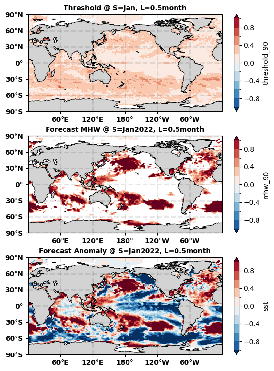
The first map above shows the threshold for initial time = January and lead time = 0.5month. The second map shows the marine heatwave detected in the NMME SST forecast at initial time = Jan 2022 and lead time = 0.5month. The third map shows the original NMME SST forecast at initial time = Jan2022 and lead time = 0.5month.

Comparison between the first and second maps shows that all identified marine heatwave signals (second map) are all higher than the threshold (first map). Comparison between the second and third maps shows that all masked regions (second map) values lower than the threshold (first map).

calculate MHW event

After the quick senitiy check, we can

• Assign Not a Number to masked our region (as no MHW)

• Assign 1 to regions with values (as MHW exist) in ds_mhw

da_mhw_event = (ds_mhw.isel(S=0,L=11).mhw_90/ds_mhw.isel(S=0,L=11).mhw_90)

Here, we picked lead time = 11.5 months to demonstrate the result of marine heatwave identification.

da_mhw_event.max()

<xarray.DataArray 'mhw_90' ()>
array(1., dtype=float32)
Coordinates:
    L        float32 11.5
    S        object 2022-01-01 00:00:00
    month    int64 1

xarray.DataArray

'mhw_90'

• 1.0

  array(1., dtype=float32)

• Coordinates: (3)
  • L
    ()
    float32
    11.5

    pointwidth :

    1.0

    standard_name :

    forecast_period

    long_name :

    Lead

    gridtype :

    0

    units :

    months

    array(11.5, dtype=float32)

  • S
    ()
    object
    2022-01-01 00:00:00

    array(cftime.Datetime360Day(2022, 1, 1, 0, 0, 0, 0, has_year_zero=True),
          dtype=object)

  • month
    ()
    int64
    1

    array(1)

• Indexes: (0)
• Attributes: (0)

As you can see from the result above that the maximum value is now 1 indicating the existence of a marine heatwave.

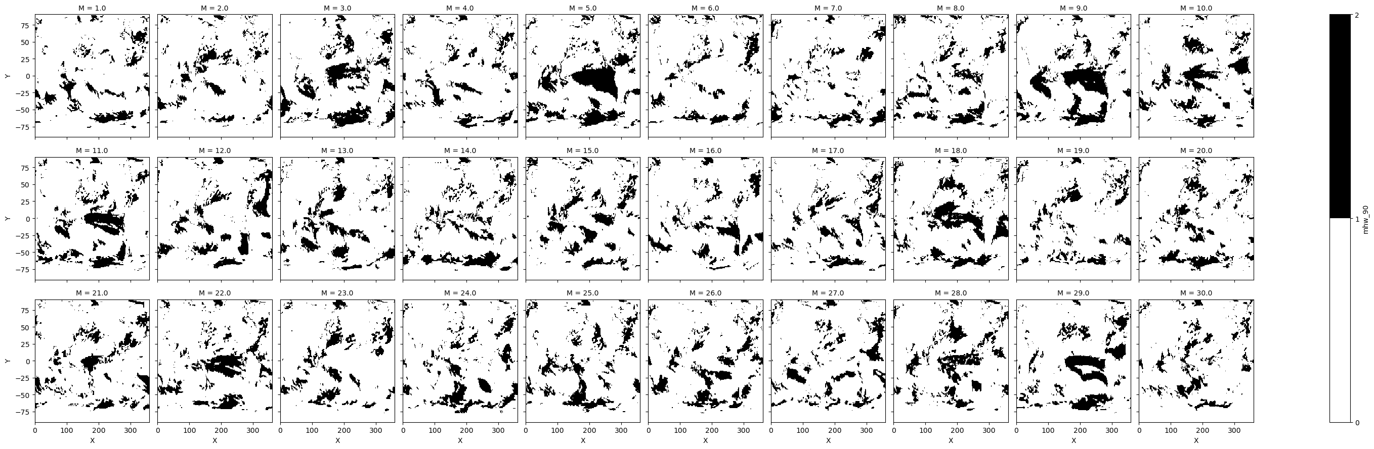
Show all enesemble member identified MHW

To show how different ensemble members can have very different results, we use the .plot() method without much formatting for a quick view of the variation between members.

Note

The following figures are for a specific start time (S = 2022 Jan) and lead time (11.5 months = 2022 Dec)

da_landmask = da_model_forecast.isel(L=0,M=0,S=0)/da_model_forecast.isel(L=0,M=0,S=0)
da_mhw_event.plot(x="X",y='Y',col='M',col_wrap=10,cmap='Greys',levels=np.arange(0,2+1))

<xarray.plot.facetgrid.FacetGrid at 0x7f36dee9ddf0>

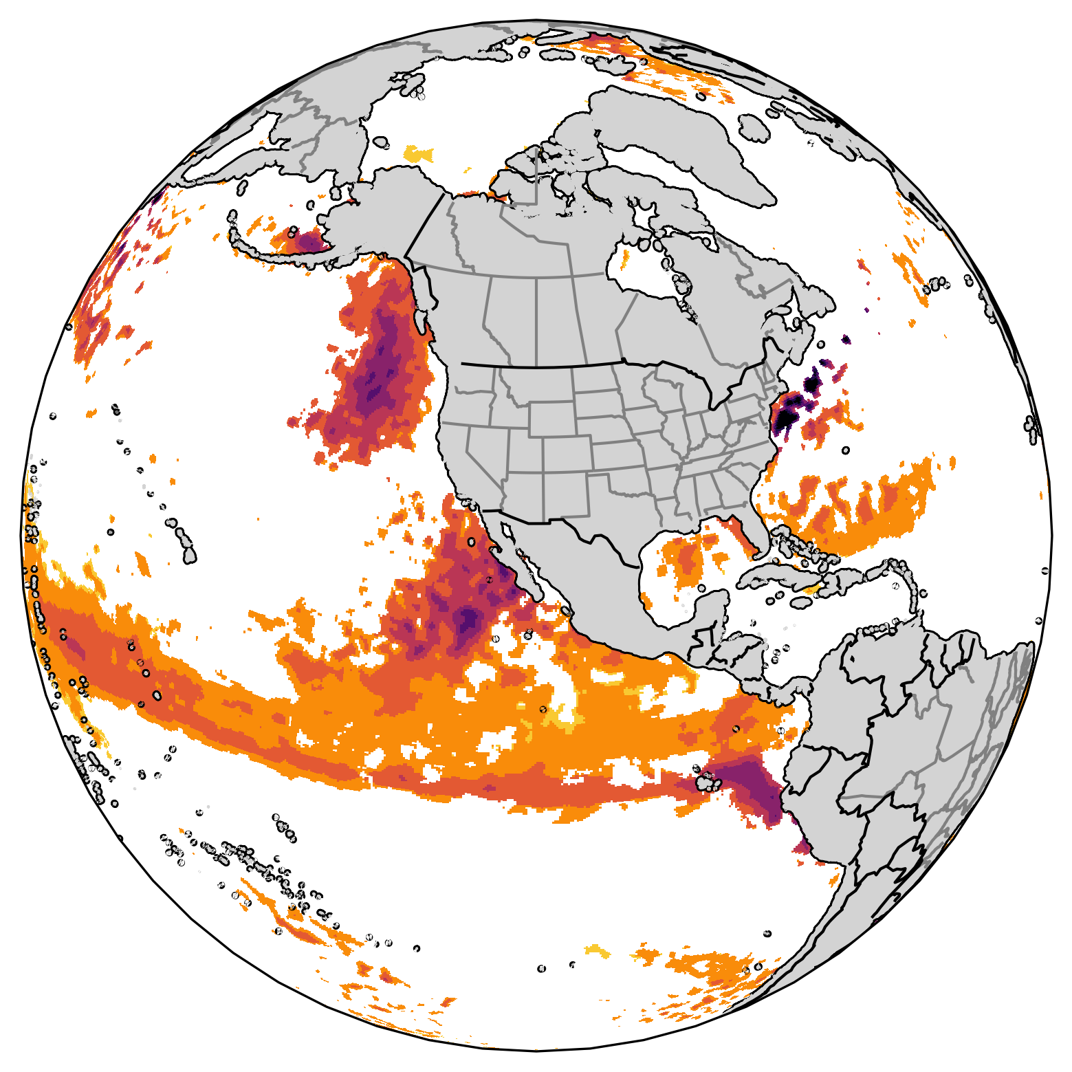
Show total identified MHW in ensemble and associated probability

By summing up all the ensemble members’ results in da_mhw_event, we know at a specific start time (S = 2022 Jan), lead time (11.5 months = 2022 Dec), and grid point how many ensemble members have predicted the existence of marine heatwaves. We divide this total number of marine heatwaves by the total number of ensemble members to produce the probability(%) of marine heatwaves in the forecast.

Important

By doing the same calculation for a different model which also has its ensemble members, we can combine the total number of marine heatwaves from across models to get a probability forecast that considers the variations between different models.

# comparing zos  
import cartopy.mpl.ticker as cticker
import cartopy.crs as ccrs
import cartopy.feature as cfeature
import matplotlib.pyplot as plt

fig = plt.figure(2,figsize=(15,15))
fontsize = 10
num_level = np.arange(0, 30+1, 5)
level = np.arange(0, 1+0.1, 0.1)

# mhw event figure
ax2 = fig.add_axes([0,0.5,0.5,0.20],projection=ccrs.PlateCarree(central_longitude=180))
im = (
    (da_mhw_event.sum(dim='M')*da_landmask)
        .plot.pcolormesh(
            x='X',
            y='Y',
            ax=ax2, 
            levels=num_level, 
            extend='both', 
            cmap='viridis',
            transform=ccrs.PlateCarree(central_longitude=0)
        )
)
ax2.set_title('Number of MHW event in ensemble members @ S=Jan2022, L=11.5month', color='black', weight='bold',size=fontsize)
ax2 = plot_format(ax2,font_size=fontsize)

# mhw probability figure
ax3 = fig.add_axes([0,0.25,0.5,0.20],projection=ccrs.PlateCarree(central_longitude=180))
im = (
    (da_mhw_event.sum(dim='M')/da_mhw_event.M.max()*da_landmask)
        .plot.pcolormesh(
            x='X',
            y='Y',
            ax=ax3, 
            levels=level, 
            extend='both', 
            cmap='plasma_r',
            transform=ccrs.PlateCarree(central_longitude=0)
        )
)
ax3.set_title('Probability @ S=Jan2022, L=11.5month', color='black', weight='bold',size=fontsize)
ax3 = plot_format(ax3,font_size=fontsize)

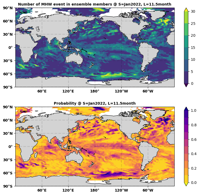
The first map above shows the total number of marine heatwave events in all 30 members of members from GFDL-SPEAR at initial time = January 2022 and lead time = 11.5month. The second map shows the probability of marine heatwave based on the NMME SST forecast at initial time = January 2022 and lead time = 11.5month. The second map is determined by dividing 30 on the first map.